The VUT equation — described by John Kingman in 1961 — is one of the most important formulas in production management. And one of the least known. I keep encountering the same pattern in client conversations and when analysing factory processes: machines running at 90–95% utilisation, KPIs looking solid, and yet lead times growing, warehouses filling up, and the planning team firefighting every day. This article explains why — and what the physics says you can actually do about it.
Source: Factory Physics for Managers — Hopp, Spearman, Jacobs. A book every operations leader should read at least once.
01 LEAN: THE EFFICIENCY TRAP
Lean Manufacturing focuses on value-added time — the te (effective process time): the actual time a machine is cutting, welding, or assembling. In practice, te accounts for 5–20% of total cycle time. The remaining 80–95% is queue waiting time — CTq.
Lean eliminates waste in te superbly. But it rarely asks the question: why does a part spend 3 days waiting before a 4-minute operation? That question belongs to Factory Physics.
02 WHAT IS CYCLE TIME?
In Factory Physics, cycle time (CT) is the total time a job spends in the system — from order release to completion. It consists of two components:
te (effective process time) — value-added time, what Lean optimises.
CTq (queue time) — time spent waiting. This is where 80–95% of total cycle time hides.
Little's Law ties it all together: WIP = CT × Throughput. Want to cut lead time? Cut WIP or increase throughput. Want to cut WIP? Cut cycle time. It's a closed loop — and the VUT equation tells you exactly what controls CTq.
03 THE VUT EQUATION
John Kingman proved in 1961 that queue waiting time in a production system is governed by three factors:
of demand & process
u/(1−u)
average te
The critical factor is U = u/(1−u), where u is actual utilisation (0–1). This is not linear — it's a hyperbola. At 70% utilisation, CTq multiplier is 2.3×. At 95% — it's 19×. The queue doesn't grow gradually. It explodes.
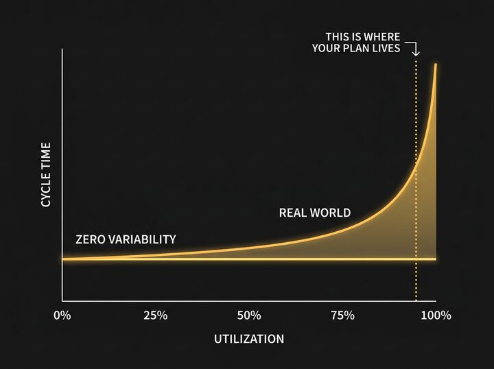
MRP/ERP planning systems often release orders requiring 120–130% of nominal capacity. Machines physically run at 85–90% — but the planning system doesn't know about physics. The queue grows silently. Work-in-process piles up. Lead times stretch. The planning system doesn't understand physics.
04 THREE BUFFERS
Factory Physics states clearly: every production system absorbs variability through one of three buffers. There is no fourth option. The only question is which one you choose — consciously or by accident.
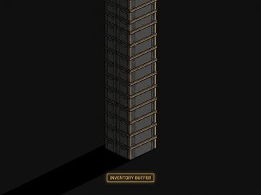


Most factories run with the time buffer — without realising it. The customer waits. The system looks "fully utilised". Management is satisfied. The market is not.
05 LITTLE'S LAW
Little's Law (1961): WIP = CT × Throughput. Rearranged: CT = WIP / Throughput. This means that if you want to reduce cycle time (lead time), you have exactly two levers: reduce WIP or increase throughput. That's it. No other variables.
In practice: a factory running continuous improvement programmes for years but never limiting WIP release will never achieve short, predictable lead times — even with perfect Lean. The physics simply doesn't allow it.
06 WHAT TO CONTROL
The VUT equation tells us precisely what a production manager can actually influence:
V — reduce variability. Standardise processes, stabilise demand, improve maintenance (fewer breakdowns = lower V). Every SMED and TPM project reduces V.
U — don't drive to 100%. The most expensive production systems are those running at 95%+ utilisation with high variability. The VUT equation proves that with mathematical precision. A strategic capacity reserve isn't waste — it's a buffer cost that's often cheaper than inventory or time buffers.
T — work on process time. Every reduction in te reduces CTq proportionally. Classic Lean territory.
When someone tells me "we have good Lean, but lead time keeps growing" — the answer is almost always hiding in one of these three questions. The most expensive things in operations don't appear on any invoice.